Designing a real-time predictive laptime algorithm for a custom in-car lap recorder.

What is a “Lap Recorder”?

A lot of racecar analytic data - about lap times, driver inputs and racing lines etc - can be derived using just a high rate GPS receiver. Which typically output position and velocity measurements at ~5-10Hz.

Hardware for collecting this telemetry often performs storage and displays real-time performance metrics as well.

EG: Racelogic VBox

A friend and I made one with an ESP32 and a small LCD screen, and I implemented the real-time performance metrics.

Scroll to bottom for hardware details and race footage!

Predictive Laptime

One useful and common metric is “predicted laptime”.

The definition of predicted laptime, for the purpose of this project, is defined as:

If the remainder of your current lap was done like the reference lap, what would that laptime be?

You might be familiar with laptime prediction from the “lap delta” estimates on video games or race broadcasts. It is usually shown as seconds relative to the best/reference lap, so the user doesn’t have to remember typical lap times for that track.

This value is very useful in real time.
For example, if the value becomes more positive during a corner, you can be confident your strategy for the corner is worse than your best.

Also useful, especially for slower cars like ours, is a velocity delta value. Returning the difference between your current speed and the equivalent point in your reference lap.

Algorithm Details

The process for predicting laptime is as follows:¹

1. New GPS position and velocity states² are captured
2. The stored best/reference lap is queried to find the time in the reference lap where the vehicle was at a comparable point
3. The time remaining after this point in the reference lap is added to the current laptime

For step 2, two decisions need to be made. Reference lap representation and comparable point definition.

We’ll start with selecting lap representation, as this also heavily informs the algorithm for finding the comparable point.

Lap Representation

If we assume that reference laps consist of GPS position and velocity values. Then the simplest way to represent the lap would be to find the most suitable GPS sample from the reference lap and do all operations with that sample directly.

Unfortunately, the resolution from this is not high enough for accurate lap times, and interpolation between samples is required.
IE: transforming the discrete GPS samples into a continuous line approximating the vehicles path.

The simplest method is linear interpolation between each sample.

A more complex method is “kinematic interpolation”, which takes velocity data and assumes a constant acceleration to increase accuracy.³

I’ve compared the two here:

Here is the above kinematic interpolation formula for a single axes, all terms but \(t\) are constant during interpolation.
\(f(t) = \mathtt{x0} + \frac{t^{3} \left( 2 \mathtt{x0} - 2 \mathtt{x1} + \mathtt{v0} \Delta + \mathtt{v1} \Delta \right)}{\Delta^{3}} + \frac{t^{2} \left( - 3 \mathtt{x0} + 3 \mathtt{x1} + \left( \mathtt{v0} - \mathtt{v1} \right) \Delta - 3 \mathtt{v0} \Delta \right)}{\Delta^{2}} + t \mathtt{v0}\)

I went with the kinematic interpolation, because it improves performance, and makes the algorithm more interesting to me!

Equivalent Lap State Algorithm

As explained earlier, when each new GPS sample arrives we need to “cut” our stored reference lap at a representative time within the lap.

The reference lap time that “represents”, or matches the new position and velocity we’ve received most closely is open to interpretation.

I see at least two approaches:
Finding the time during the reference lap that is…

1. Closest overall to the new sample, a simple 2D distance calculation ignoring current velocity
2. Closest to the lateral axis, finding the point on the reference lap that lies on a line perpendicular to the current heading

I’ve compared the two approaches here:

The graph also shows a nonlinear solver trying to locate the intersection as in Method 2. It’s initial guess is 0.5.

Things to note:

• The distance curve from Method 1 looks harder to solve, the inflection point will likely take more evaluations to find.
• Method 1 is also more vulnerable to false convergence, you don’t know you’ve found the best solution available. Whereas for Method 2 any solution is okay.
• For Method 2, multiple solutions will exist, as the tracks are usually loops. But if you start your search at the previous solution, you should hit the correct one reliably.
• For Method 2 in a corner, it might not be correct to say that one car on the inside and one on the outside are “comparable”. But we can more easily assume lateral position on a straight doesn’t have an impact. And drivers should be too busy to read the value during a corner anyway!
• This example is contrived with a huge change in direction. For more realistic data the curves will become more linear, and the solution will take fewer iterations to find.
• In a corner, Method 1 and Method 2 may produce different results. As is the case in the visualisation.
• Method 2 will become less predictable and accurate if the vehicles heading is erratic.

I went with Method 2, because it seemed much more amenable to computational solutions.

To use a nonlinear solver we need a formula for the distance between a point (the position returned by our interpolation above), and a line perpendicular to a given angle.

\(f() = \left( - \mathtt{Px} + \mathtt{tx} \right) sind\left( \mathtt{heading} \right) + \left( - \mathtt{Py} + \mathtt{ty} \right) cosd\left( \mathtt{heading} \right)\)
Source

I’ve modified the formula so that it takes heading angle, (which is 90 degrees from line angle) and to ensure distances in the “heading” direction are positive.

The interpolation formula is substituted into the distance formula to produce a very large equation⁴ used in the plot above.

This equation should reach 0 when the time from the reference lap produces a vehicle position that lies on a line perpendicular to the vehicles heading.

The Implementation

Considerations:

• The formulas are very large, so I used Julia to do the substitution and autocoding to C.
• The ESP32v3 only has hardware support for floats, not doubles. So I needed to be careful to use the fpow instead of pow, for example. To ensure all the floating point maths is accelerated.
• Generating test data to test the algorithm on a laptop was invaluable. Debugging on target is very hard for maths problems.
• Uses the -Ofast clang argument, fusing floating point operations and reducing instructions by two thirds.

Contact me for some of the code, if you’d like to see it.

The Hardware

• ESP32 v3
• Arduino SDcard shield
• Ublox 10Hz GPS module, with external antenna
• Screen from an old 3d printer
• AA batteries
• A rustic 3D printed enclosure

The installation process is simply drilling holes in the dashboard, and applying cable ties until it seems like it’s not going anywhere:

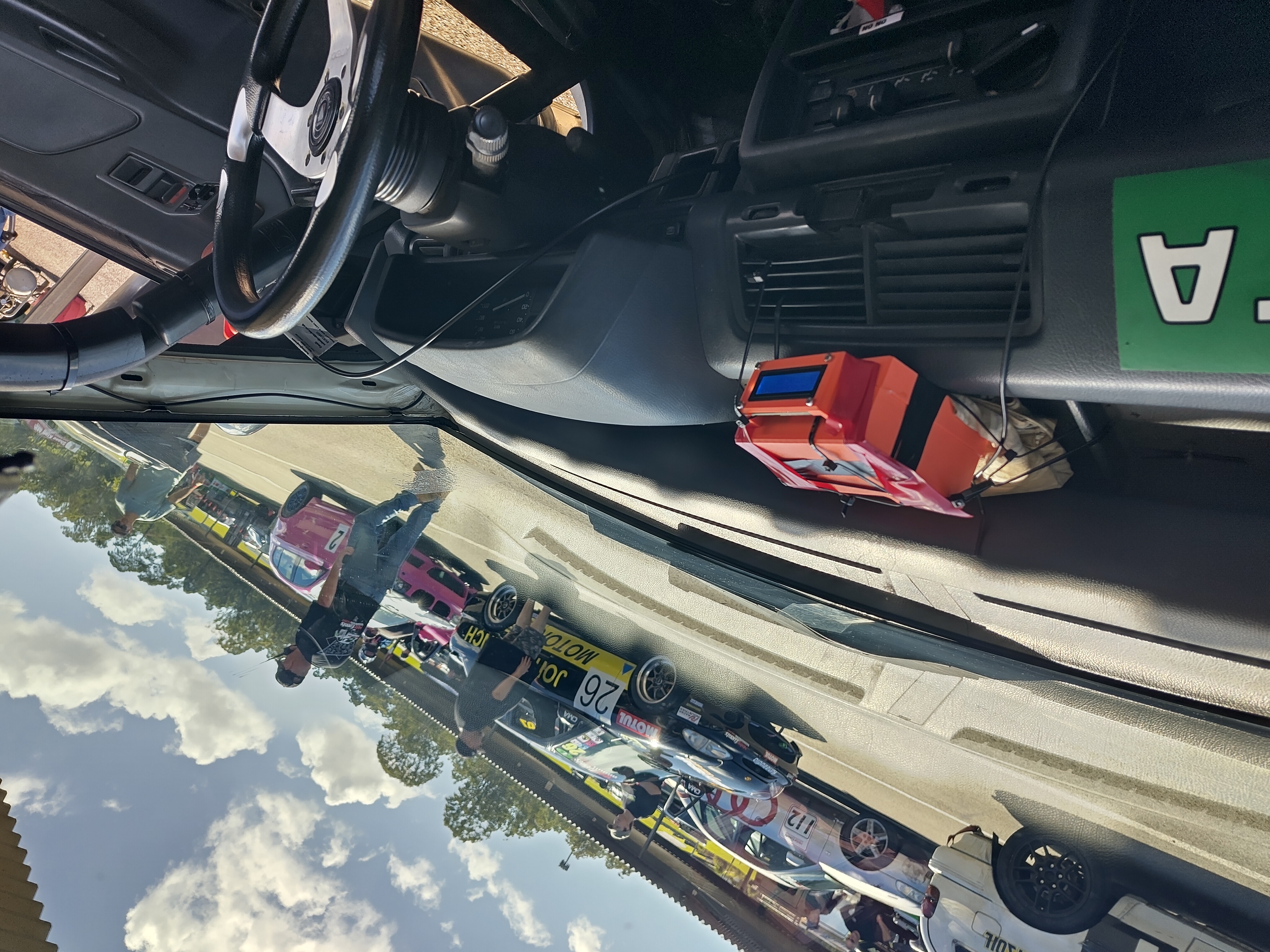
Unfortunately it did go somewhere, although as the day progressed we cobbled it back together:

(I’m the driver who didn’t notice their gloves were missing… Woops!)